Wavefront Errors and the Origin of Adaptive Optics
This page is an overview of adaptive optics and its applications from high intensity lasers to microscopy and retinal imaging. Learn how deformable mirrors are used to compensate for wavefront errors and help imaging systems go from blur to clarity.
Optical systems performance is directly linked to the amplitude of wavefront distortion along the optical path.
For example, a classical imaging system such as an objective lens, is typically considered “high performing” if the wavefront error (wfe) introduced by its lenses is minimal (typically wfe < Lambda/20 rms). It is also qualified as “diffraction limited,” meaning the resulting point spread function is close to the perfect Airy function. Optical designers from various industries make great efforts to calculate combinations of lenses or optics to reduce this wfe. For imaging lenses or optical components, the wavefront error is fixed and comes from the system itself, from its design on one hand, and errors of fabrication on the other hand. In other cases, wavefront distortion can come from other sources along the path, with time or space dependency. For example:
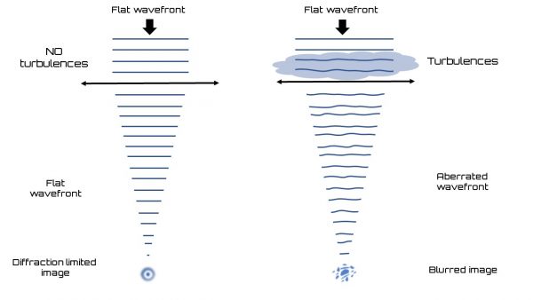
-In astronomy, (see fig 1 below) because of atmospheric turbulences, a perfectly designed telescope, (i.e. with minimal aberrations) will still generate blurry images.
-In high intensity or high energy lasers, the high power of the beam passing through optics causes time and space dependent index refraction changes that highly distorts the focal spot.
-In fluorescence microscopy, depth dependent index changes of biological tissue induces aberrations that makes the imaging or fluorescence excitation inefficient and distorted at a certain depth.
-In retinal imaging: the patient eye itself creates aberrations which greatly limits the final resolution of the retina image acquired.
Figure 1: Impact of turbulences on the wavefront error
What is Adaptive Optics?
The idea behind adaptive optics is to compensate for these distortions and recover the system resolution. Originating from astronomy, the idea of adaptive optics was first introduced by the American astronomer Horace W. Babbock as early as 1953 for the correction of atmospheric turbulences.
The first AO system based on a wavefront sensor, wavefront reconstructor and deformable mirror comparable to those used today was developed in the early 70s within the scope of a DARPA agency grant aiming at imaging and tracking satellites. The RTAC (Real Time Atmospheric Compensator) developed in association with the company ITEK, MA was first demonstrated in 1974 [Hardy and al.] and the first implementation of an AO system (CIS – Compensated Imaging system) was made on a 1.6 m telescope located on Mt Haleakala on Maui Island. This system was associating a piezoelectric DM with 168 actuators, separate Tip-Tilt Correction and an intensified shearing interferometer as a wavefront sensor, all together able to perform closed loop correction up to 1000Hz.
In the early 90s, several astronomical agencies such as the National Optical Astronomy Observatory (NOAO), the European Southern Observatory (ESO), and Office National d’Etudes et Recherches Aerospatiales (ONERA) in France started their own developments aiming at astronomy applications.
How Do Adaptive Optics Systems Work?
Adaptive optics (AO) systems consist of measuring and compensating distortions in the incoming wavefront in order to recover signal or resolution. The wavefront measurement is typically performed with a wavefront sensor such as a Shack-Hartmann wavefront sensor, whereas the compensation is carried out by a deformable mirror. A control system or software will then apply a closed loop algorithm and the ensemble will provide a corrected output wavefront which can then be processed by detectors or cameras. Adaptive optics systems have demonstrated significant resolution improvement. With the recent progress in camera technologies, wavefront sensors, deformable mirrors and real time computers, AO systems have become very popular and are now used in many fields such as high-power lasers, free space optical telecommunications, micro and nano-manufacturing, fluorescence microscopy, optical coherence tomography and retinal imaging, just to name a few.
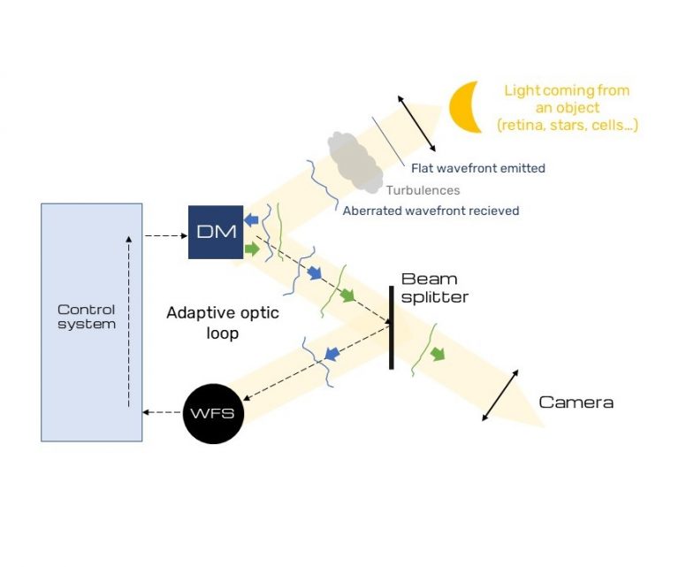
Figure 2: Adaptive optics closed loop: using a deformable mirror to correct the wavefront error
The figure to the left illustrates the working principle of a close-loop adaptive optics for astronomy.
The wavefront from a distant object under observation, typically a star, is distorted by atmospheric turbulences. A part of the beam is directed to a wavefront sensor which measures the wavefront error of the incoming wave. The control system processes this measurement and sends a command to the deformable mirror to change its shape and compensate the distortion. The resulting output beam is now corrected and sent to the science camera for imaging.
By continuously measuring and correcting wavefront errors in a loop, the adaptive optics system constantly produces much sharper and clearer images than would normally be possible to acquire.
Adaptive Optics Loop Components
An adaptive optics loop is typically composed of 3 major components:
– A Wavefront Sensor
Wavefront sensors provide the 3D map of the optical wavefront or phase front with speeds up to several KHz. They quantify atmospheric disturbance, or optical aberrations with a high precision of λ/100 RMS. Shack-Hartmann wavefront sensors are by far the most used sensors for adaptive optics, because they are easy-to-use, accurate, fast and robust. Other types of sensors can also be used depending on the application. For a list and description of wavefront sensors, please click here.
– A Deformable Mirror or Spatial Light Modulator
Deformable mirrors are mirrors with electronically controlled surface shapes. They are commonly used to compensate aberrations. They can be based on piezoelectric transducers, mechanical or electromagnetic actuators. Spatial Light Modulators with phase modulation are high resolution arrays that can control the phase of the optical wavefront, pixel by pixel. Although they present lower spectral bandwidth and smaller damage threshold, they have much higher resolution than deformable mirrors and can especially be used for beam shaping applications. For a list and description of deformable mirrors, please click here.
– Control Software/Algorithm (closed loop or open loop)
The Adaptive Optics control software is in charge of controlling all the components of the AO loop, receiving signals from the wavefront sensor and computing the right commands to send to the deformable mirror. In a lot of cases, a closed loop approach is chosen to compensate for time dependent aberrations (such as atmospheric turbulences). However, when wavefront sensing becomes very challenging, an open loop approach could also be chosen, for example in microscopy.
In this application note, among the many examples of adaptive optics implementation, we choose to describe only the following few examples:
-Directed energy weapons
-High energy and ultra high intensity lasers
-Microscopy and ophthalmology
Adaptive Optics for Directed Energy Weapons, High Energy and Ultra-high Intensity Lasers
Directed Energy Weapons
Directed-energy (DE) weapons have been in development for the past three decades. On one hand, high energy lasers (HELs) offer many advantages over conventional weapons, including the delivery of energy at light speed, a low cost per shot, unlimited magazines, and stealth. On the other hand, the performance of DE weapons is dependent on atmospheric conditions. This is why adaptive optics have a key role in those developments in order to optimize the irradiance on target, by compensating the aberrations coming from the laser (thermal effects), the optical train (beam transportation optics) and of course from the turbulence along the emitter to target optical path.
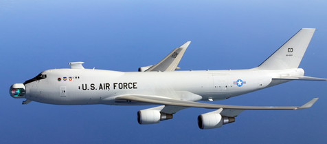
Figure 3: Airborne Laser (ABL) anti-ballistic missile weapons system
DE weapons have been tested in the field, in air, on land and in the sea. Although those developments and applications are understandably classified, it is possible to find some literature describing the motivations and models. For example: “Adaptive Optics for Directed Energy: Fundamentals and Methodology” (here).
High Energy and Ultra High Intensity Lasers
High energy lasers for nuclear fusion - Inertial Confinement Fusion (ICF)
Nuclear fusion is expected to become one of the next big technological breakthroughs in the coming decades. The utilization of high energy lasers for nuclear fusion is well on its way, and will hopefully allow us, one day, to produce low cost “clean energy” in the near future.
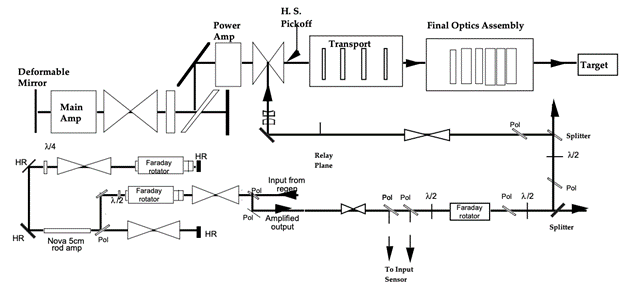
Inertial Confinement Fusion (ICF) is a process that uses lasers to heat a small micron size target in order to produce energy through the fusion process. This approach was validated in the USA with the OMEGA and NOVA lasers in the late 70s and 80s but the first real milestone was achieved on December 5, 2022 at the NIF facility at the Lawrence Livermore laboratory where 192 beamlines combined delivered 2.05MJ of UV (351nm), over a few ns, which resulted in producing 3.15 MJ of energy – more energy than the target had received.
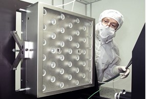
Each beamline of the NIF includes an adaptive optics system, with the deformable mirrors being located at the end of the main amplifier, correcting residual thermal distortions, imperfect optical materials and amplifier distortions due to flash lamp heating. This wavefront correction allows to achieve smaller spot size and produce higher power density on the target, therefore facilitating the fusion process.
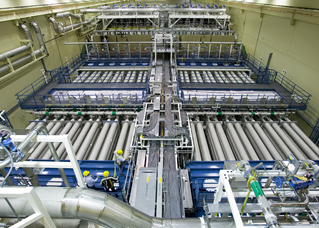
Figure 6: Example of a NIF beam line
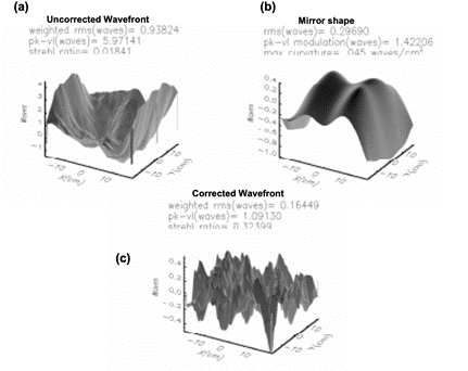
Figure 7 below shows the wavefront correction of the NIF baseline design. The aberrated wavefront of the uncorrected beam (a) is compensated by DM shape (b). The residual (c) shows a 6-fold decrease of the WFE amplitude and 18x increase of the strehl ratio.
Figure 7: Correction of the wavefront errors of the NIF baseline design
The promising results obtained at the NIF triggered a flood of investments into private companies promising to deliver fusion power in the 2030s and the use of adaptive optics for high energy lasers is therefore expected to grow.
Focal Spot Optimization for Ultra High Intensity Lasers (UHIL)
The number of facilities employing ultra high intensity lasers have been on the rise since the late 90s. Those sources typically use mode locked oscillators that are amplified to produce femtosecond type pulses with peak power varying between 10s of TW to several PW on target. This paves the way for experimental production of extreme electromagnetic conditions required for relativistic physics. Not only are those sources more compact and cheaper to build and assemble than linear accelerators and synchrotrons, they are also much easier to operate and maintain.
Adaptive Optics brought major improvements to UHIL facilities, allowing the lasers to deliver quasi theoretical maximum intensity on target.
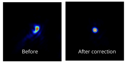
Unlike in astronomy, the speed of wavefront correction in UHIL is not critical and the key factors are rather the optical quality of the deformable mirror, the performance of the wavefront sensor and the ability to optimize the final spot. Figure 9 shows a focal spot before and after adaptive 0ptics correction obtained at the Laboratoire Irène Joliot-Curie, Université Paris-Saclay in Orsay, France. The adaptive optics system used was composed of an ILAO-Star deformable mirror, a HASO wavefront sensor and the Wavetune software from Imagine Optic.
Figure 8: Courtesy of Bella Petawatt laser system
Historically, bimorph and monomorph deformable mirrors, developed for directed energy and astronomy, were the only large deformable mirrors available until Imagine Optic introduced its new line of ILAO mechanical deformable mirrors.ILAO and ILAO Star are specific DMs developed for UHIL applications. They meet all critical requirements for UHIL: large aperture, optical quality (1o nm rms active flat), extreme stability (no drift) and quasi perfect linearity. Figure 10 shows a 400 mm diameter ILAO STAR – custom designed for petawatt femtosecond laser manufactured by Imagine Optic.
Figure 9: Courtesy of UHIL 100 CEA Saclay (100TW, 25 fs, 10 Hz) with strehl Ratio improvement from 0.45 to 0.87 with AO kit ILAO from Imagine optic
Figure 10: 400 mm substrate ILAO STAR - custom designed for petawatt femtosecond laser by Imagine Optic - Credits Alok Kumar Panday
Adaptive Optics for Microscopy
Adaptive Optics is commonly used in several microscopy techniques such as non linear two photon microscopy, confocal microscopy, light sheet microscopy and superresolution microscopy (PALM/STORM). One of the biggest challenges in applying adaptive optics to microscopy is measuring the disturbed wavefront at the desired location. For example if the goal is to get a perfect beam focusing at a certain depth of the sample, how could we measure the wavefront inside the sample? Scientists have come up with different tricks to perform this measurement, in some cases, guide stars are used or generated inside the sample to run a closed loop. In other cases, open loop algorithms were implemented. This sections provides examples of different AO implementation schemes.
Multiphoton, non linear microscopy
Multiphoton microscopy is an alternative to laser-scanning confocal microscopy. It uses the same principle of scanning the excitation beam over the sample, but differs to the extent that it is using a multiphoton excitation beam to create the fluorescence signal. This technique is broadly used for in-vivo imaging or deep imaging because it minimizes background fluorescence signal, overcomes to some extent scattering of sample tissues and is less photo-toxic than conventional confocal techniques. However, as the imaging goes deeper in the tissue, optical aberrations quickly become significant, which destroys the quality of the focal spot and reduces the 2P signal generated drastically. Adaptive optics was proven to be a good solution to recover performance when imaging deep, with better, tighter focus, improved axial sectioning, resolution and 2P signal emitted with typical x2 to x5 gains obtained. Perhaps the most well known microscope with adaptive optics is the one developed by Betzig and Wang at Janelia farms published in 2014 (click here to access it). Two subsequent advantages of adaptive optics and the signal gain are: 1) the ability to reach much deeper layers of the sample and 2) to decrease the intensity of the excitation laser, therefore reducing photo-toxicity. Below are two examples of adaptive optics applications to 2P imaging that have been published. In the example 1 below, AO is implemented on the excitation path of the multiphoton microscope. An iterative algorithm was used to optimize the DM shape to get the most signal.
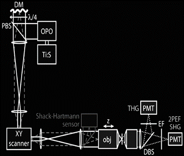
Example 1: Drs. Beaurepaire, Débarre & Olivier, Ecole Polytechnique, France, 2012
Figure 11: Multiphoton microscope setup with adaptive optics implemented on the excitation path
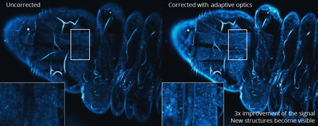
Figure 12 is an image of a drosophila larva acquired with this microscope (Court. of Drs. Beaurepaire, Débarre & Olivier, Ecole Polytechnique, France, 2012). We can see a 3x improvement of the SNR thanks to AO.
Figure 12: images of drosophila tissues acquired with that same microscope at about 30µm, depth, without (left) and with (right) adaptive optics
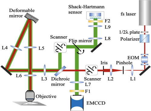
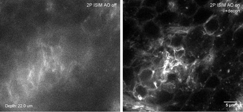
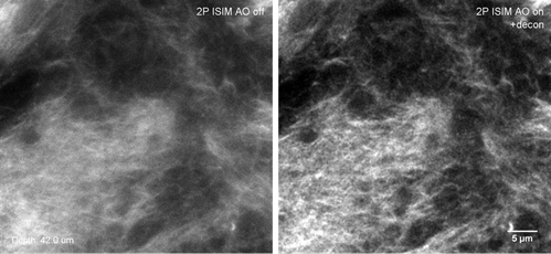
Example 2: Wei Zheng, Yicong Wu, Peter Winter & Hari Shroff, NIH, 2017
In this second example of AO implementation in a multiphoton set up, the deformable mirror is on the excitation and emission path. The wavefront measurement is carried out on “descanned” guide star. A flip mirror directs the light onto a wavefront sensor or the imaging camera (Court. of Wei Zheng, Yicong Wu, Peter Winter & Hari Shroff, NIH, 2017).
Figure 13: multiphoton setup where AO is implemented (Court. of Wei Zheng, Yicong Wu, Peter Winter & Hari Shroff, NIH, 2017)
Figure 14: images of drosophila tissues acquired with the microscope described on Figure 13 at 2 different depths ( 22µm, 42µm) without (left) and with (right) adaptive optics.
Adaptive Optics for Retinal Imaging
Ophthalmology has immensely benefited from the use of adaptive optics. Human eyes are very imperfect optical elements: they present irregularities which introduce aberrations and distort light waves. As a consequence, retinal examinations have always been limited to a rather low level of details and early signs of diseases occurring at the level of cells, had remained invisible to eye doctors.
One example of successful implementation of adaptive optics for retinal imaging was performed by the company Imagine Eyes. Figure 16 below shows a real time image of a live retina with adaptive optics ON and OFF. The system drastically improves the resolution and provides instant visualization of cellular details (rods and the cones) of the retina.
Figure 15: Retinal Imaging using Rtx1 from Imagine Eyes to improve the resolution: see the difference when the AO is ON.
Adaptive Optics for Satcom and Free Space Optical Communications (FSO)
Adaptive Optics (AO) removes the effect of air turbulence in order to improve the coupling efficiency in the receiver optical fiber. Typically, an AO system allows an optical gain of at least 10x on the injected flux which translates into a 10 fold increase in link capacity.
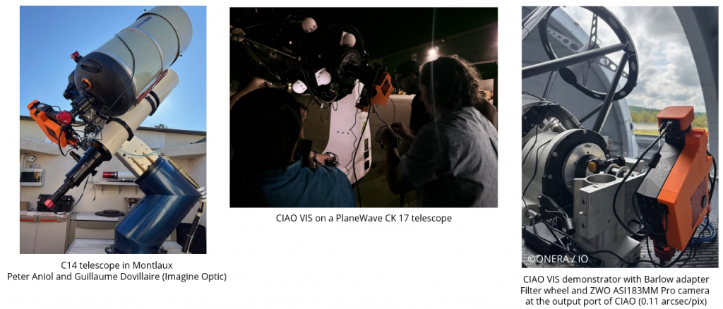
Our partner Imagine Optic offers a standard turn-key system called CIAO SWIR that integrates all components into a telescope compatible package. CIAO SWIR was designed with affordability in mind, and is based on an efficient and fast DM/wavefront sensor/Software combination.
CIAO exists also in a visible version, allowing astronomers to do high resolution imaging: more about CIAOhere.
Stay tuned for regular updates as we keep pace with the ever-evolving landscape of Adaptive Optics technology. This page is dedicated to serving as a comprehensive resource for applications in adaptive optics, ensuring you stay informed of advancements. Check back frequently for the latest updates and insights.