RCM2 & RCM2.5 | Point-Scanning Confocal Microscopes
Rescan confocal microscope is an easy to use, sensitive, high
Rescan confocal microscope is an easy to use, sensitive, high
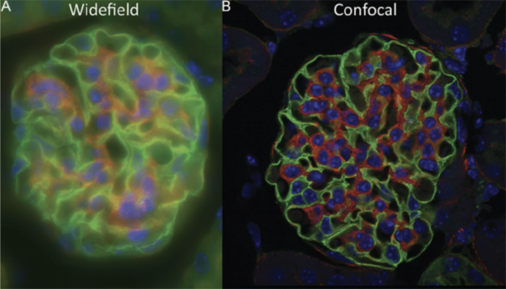
Confocal microscopy is an optical imaging technique that uses spatial filtering (in most cases a pinhole), to block the out-of-focus light from physically reaching the sensor – in other words, optical sectioning. Although a confocal microscope will theoretically improve the lateral and axial resolution slightly compared to a widefield microscope. It can lead to a huge increase of the optical sectioning, therefore offering much thinner and effective axial resolution.
In a widefield configuration the entire specimen is illuminated evenly, and all parts of the sample can be excited at the same time (both in the lateral direction, i.e. X-Y and in the axial direction, i.e. Z). Every fluorophore contained in that volume will emit light, and all this light will be collected by the camera no matter where it comes from. The camera collects what is called out-of-focus light, and this can drastically decrease the contrast of an image, especially for thick samples (typically bigger than 2µm) [1].
In a confocal configuration though, the light from the laser is focused onto the sample in the focus plane of the objective. Only a small area is illuminated on that plane, and because the beam is focused, the energy density is much higher at the focus plane compared to the planes above or below. Therefore, fluorophores in the focus plane are much more likely to emit light than fluorophores on the planes above or below. Nonetheless there is still some out-of-focus light being emitted.
Below is a schematic of the light path in a widefield microscope (left) and in a confocal microscope (right).
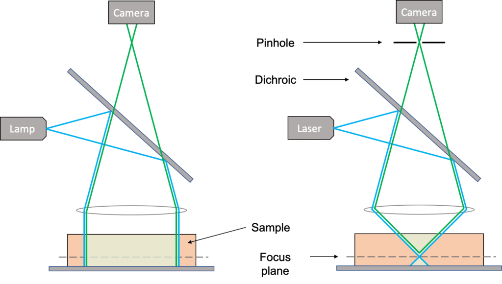
As we can see in the schematic below the pinhole blocks the light coming from the planes below or above the focus plane. So, using both a focused illumination and a pinhole, a confocal system will acquire only the light coming from the focus plane and therefore the information contained in the image only corresponds to fluorophores in that plane. Acquiring multiple planes then helps to reconstruct the 3D shape of the sample.
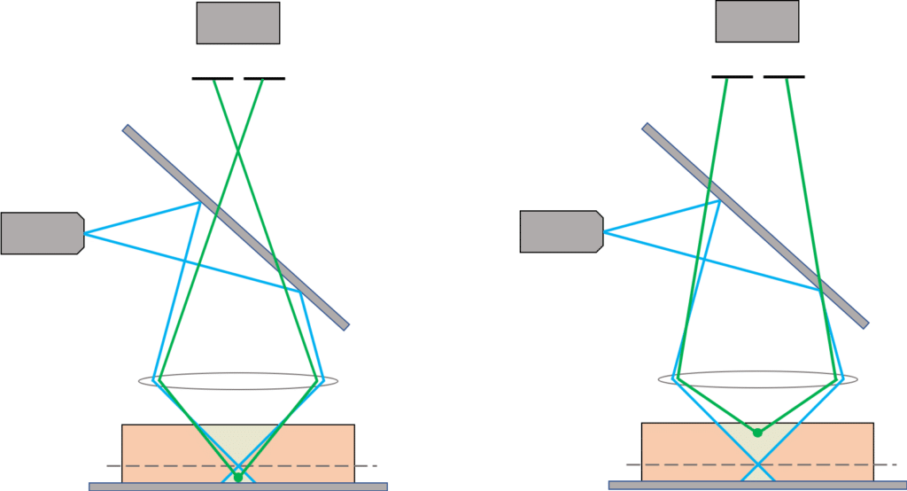
Nowadays confocal microscopes are much more complex than just a focused illumination and a pinhole, but overall, these are the two features that bring the confocal capability.
But let’s have a closer look at the first scheme comparing widefield and confocal configurations. As mentioned, a widefield microscope evenly illuminates all parts of the sample at the same time, while a confocal microscope only illuminates a small area at one time. That means that to completely illuminate the sample in one plane we need to scan the light all over the FOV (in X-Y). Therefore, confocal microscopes also feature moving mechanical parts to scan the light all over the sample. There are two main categories of confocal systems: laser-scanning confocal microscopes and spinning-disk confocal microscopes.
The most straightforward way to illuminate the whole FOV with the confocal configuration is to scan the illumination in X-Y. Microscope manufacturers do that by using scanning mirrors. Usually two mirrors: one to scan along the X direction (fast mirror) and one to scan along the Y direction (slow mirror). For every single point, the detector records the fluorescence light emitted by the sample using a “single-pixel” detector: typically, PMTs (photomultiplier tubes) or HyDs (hybrid detectors). In such a configuration the image is formed digitally after sequentially capturing the light from the sample emitted at each position of the scanners. This technique is called laser-scanning confocal microscopy.
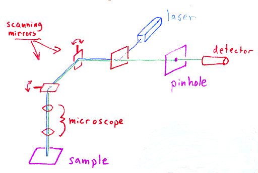
[Image from http://www.physics.emory.edu/faculty/weeks//confocal/]
Laser scanning confocal microscopy is the most widely used method for confocal imaging. The main advantages of are; the high optical sectioning (Z resolution, as good as 500nm raw data), high lateral resolution (X-Y resolution, as good as 240nm raw data), and versatility of implementations and uses (upright or inverted stands, low mag or high mag objective lenses, different samples holders types etc.). The two main drawbacks are the speed and the phototoxicity
The speed, because we need to sequentially point-scan the region of interest. Typically, the scanning speed of galvo mirrors is 1µs/pixel so for an image of 1024×1024 pixels, we need about one second to acquire one frame. This is for one plane only, however the goal of a confocal microscope is to capture the 3D structure of the sample, so we would need to acquire multiple 2D images. This can lead to acquisition time of few minutes, and sometimes hours. In recent years confocal microscopes feature a new type of scanning mirrors to increase the speed, resonant galvo mirrors.
Although those mirrors can go much faster, offering ultra-short pixel dwell-time this does not change the fact that the scanning process here is sequential so noticeably short illumination will probably lead to insufficient signal-to-noise ratio. This becomes even more noticeable considering that the detectors used in laser-scanning confocal microscopes, PMTs or HyDs are relatively not sensitive.
The phototoxicity could be a big problem on a laser-scanning confocal microscope. The main reason lies to the fact that phototoxicity is not a linear process. Therefore, applying twice the of the light intensity for half the time will create more stress and photo-damage than half the intensity for twice the time. Here is an example to understand the process better. If we want to collect as many photons from the sample in a laser-scanning confocal microscope than in a widefield microscope, assuming both systems are the same in terms of light efficiency.
For a 1024×1024, each point in the sample will be excited for about one over one million of the entire acquisition time. To collect as many photons as in a widefield system we therefore need to apply one million times more power density to each pixel than in a widefield configuration. As mentioned above, this will create much more photo-damage than in a widefield experiment. This is taking the assumption that both systems have similar light efficiency, which is generally not true, as cameras have higher QE than PMTs or HyDs.
Because of those two drawbacks (speed and phototoxicity), laser-scanning confocal microscopes are typically not the best systems to image living cells. Both because of the low temporal resolution and the photo-damage that the illumination will create on the sample.
There is another way to increase speed: parallel illumination. This technique was originally introduced 40 years ago but recent improvements in microscope designs and camera technologies have significantly expanded the potential of this technique. The spinning-disk confocal microscope consists of a disk with multiple pinholes, rotating at a very high-speed (5,000 – 10,000 rpm). The illumination is parallel before the disk. The objective lens focuses multiple scanning points onto the sample. This creates a parallel illumination by opposition with sequential scanning on a laser-scanning confocal microscope. Within one rotation, every part of the sample has been illuminated several times, offering acquisition speed up to 1,000 – 2,000 fps. Again, the limitation is most likely going to be the signal-to-noise ratio, but video rate (~30 fps) can easily be achieved.
Nowadays, spinning-disk confocal microscopes are more complex than that. They usually feature two rotating disks, the first one has microlenses in order to more efficient to inject the light into the second disk with pinholes. Furthermore, those systems are using cameras as detectors and are not technology dependent: both CMOS, CCD, sCMOS or EMCCD can be used!
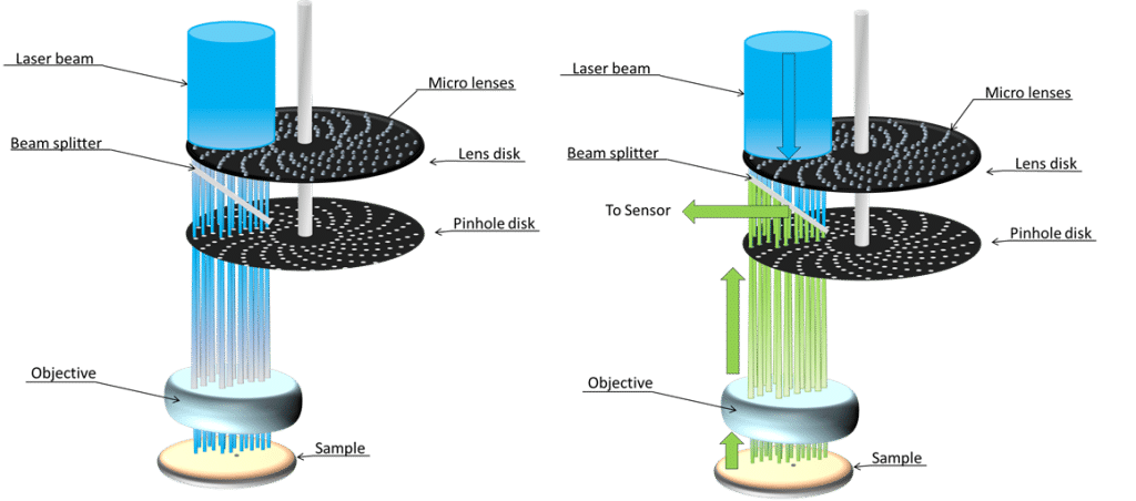
[Image from https://www.cherrybiotech.com/scientific-note/microscopy/introduction-to-spinning-disk-confocal-microscopy]
This imaging method is much more appropriate for living cells imaging. The main advantages are the high temporal resolution and the lower photo-toxicity than a regular laser-scanning confocal microscope. But there are several drawbacks, like the fact that the fixed pinhole size and as a result both the axial and lateral resolution are not optimized for each objective lens.
Furthermore, several imaging artifacts are to be considered when using a spinning-disk. First, pinhole crosstalk, the out-of-focus light can still reach the detector by travelling through adjacent pinholes. Second, low light efficiency, as most of excitation and emission light do not pass through the disks and back-reflection could increase the background of the image. Third, field inhomogeneity, which could be compensated using a liquid light guide. Fourth, the inherent limitation of selecting and scanning only a specific ROI (like for FRAP experiments). These are the most common reasons, result in choosing a laser-scanning confocal architecture over a spinning-disk confocal one.
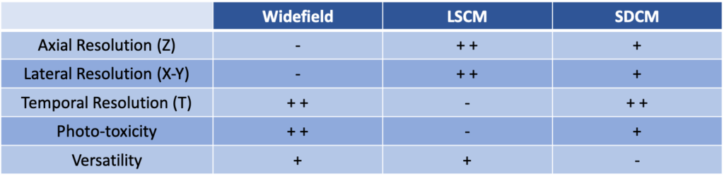
There is no perfect system, and everything is a trade-off. Confocal microscopes are the ideal solution for thick tissues, but then the imaging method will mostly depend on your sample. For fixed tissues which will not suffer too much of the photo-damage, laser-scanning confocal microscope is the ideal solution, offering higher lateral and axial resolution. However, for living cells, if you do not need the extra resolution offered by a laser-scanning confocal (LSCM) architecture, then spinning-disk confocal systems (SDCM) are the ideal solution. Chart below summarizes this section.
The Rescan Confocal Microscope (RCM) belongs to the same family of the “enhanced confocal” systems mentioned above. It is a confocal microscope, but it also beats the diffraction limit by a factor 1.4 before deconvolution (2-fold after deconvolution) and is also a super-resolution system.
The excitation part works the same as pretty much any laser-scanning confocal microscope. The sample is being point-scanned using scanning mirrors to move the beam in X-Y and cover the entire FOV. The light is being emitted, de-scanned and focused through a pinhole to get optical sectioning the same way it would on a regular laser-scanning confocal system. This is after that the magic happens. Instead of using a single-pixel detector we use a camera (typically a sCMOS) and a second pair of galvo mirrors to re-write the signal on the camera chip. Those mirrors are called the rescanners (hence the name of Rescan Confocal Microscope).
In the scenario where both pairs of mirrors have the same amplitude (scanners and rescanners), the system simply re-write the fluorescence signal of the sample onto the sensor chip of the camera. But when the rescanners have a bigger amplitude, it stretches the image in both X and Y directions. As a result, we obtain a magnified image.
Now, any optical magnification, no matter how big it is, does not increase the resolution of a system. It magnifies the image, but it magnifies the blurry function in the same way. Therefore, at the end the resolution power remains the same. But here we are not talking about an optical magnification, but a mechanical one. In the sense that this is the movement of the scanners that spread the light to a bigger area of the sensor and create the magnification. Therefore, we are not limited to the diffraction limit anymore.
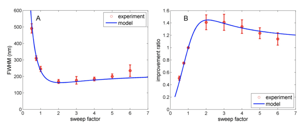
As a result of the rescanners move faster than the scanners (same frequency but higher amplitude = movement speed is faster) they introduce a motion blur in the image. That counterbalance to some extent the resolution improvement obtained with the mechanical magnification. The graph (right) below shows the resolution and improvement ratio using a 100X / NA1.4 lens at different sweep factors between the rescanners and the scanners. Sweep factor of 2 means the rescanners have twice the amplitude of the scanners. As we can see, the sweep factor of 2 is optimal for the resolution. In that case the resolution improvement due to the mechanical magnification is equal to 2. The motion blur due to the higher scan speed is only of 1.4, so the total resolution improvement equals 2/1.4 = 1.4.
This part is nicely explained in the following video. Above the 170nm lateral resolution we can run deconvolution to go down to 120nm. This is the same resolution as a SIM, Airyscan, ISIM and SoRa systems.
The resolution enhancement is only one aspect of this system. Because the RCM uses a camera as a detector, it is much more sensitive than PMTs or HyDs based systems. A typical sCMOS camera offers QE over 70% between 400-700nm with peak at 82%, and the most sensitive ones even offer peak at 95%! This is to compare to 30% at best for a PMT or 45% for a HyD detector. RCM’s optical architecture is remarkably simple. It ensures all photons that are captured by the objective lens are imaged onto the camera. As a result, the overall light throughout is very high, approximately 3-4 times higher than other regular confocal microscopes. RCM is extremely sensitive, which makes it a particularly good choice for samples like live cells.
Though the RCM remains a laser-scanning confocal system and therefore is rather slow. As a result of a precise synchronization requirement between scanners and rescanners, non-resonant scanners are the only available option. Yet this limits the speed of the system. The RCM typically runs at 1fps for 512×512. Those specs are summarized in the following chart:
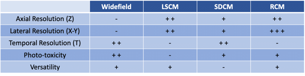
As shown in the previous chart and all over this discussion there is no perfect system. It is most of the time a question of compromise and depends on your application. If speed is not mandatory for your research then the RCM is the ideal system. It offers confocal capability, high lateral resolution, low photo-toxicity and is as modular as any laser-scanning confocal microscope (FRAP, …). The camera feature allows RCM to operate in a regular widefield configuration. This makes the workflow of finding and focusing onto the sample extremely easy. Finally, the RCM is a cost-effective solution, thanks to the simple design. It does not require expensive components (only galvo mirrors). Additionally, it is an upgrade compatible with any widefield microscope brand, and most of the cameras widely used for microscopy.
Images below shows the nuclear spread from fixed mouse spermatocytes. Immunostained for SYCP3 (a component of the synaptonemal complex) and labeled with Alexa 488. The images on the top were acquired using a regular laser-scanning confocal system with a pinhole of 1AU. The images on the bottom were acquired using the RCM with a pinhole of 1AU. On the left side we have the whole FOV before and after deconvolution. On the right side we have a zoom before and after deconvolution.
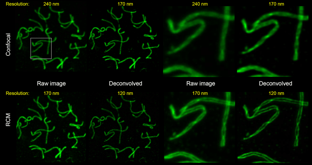
The raw data of a regular laser-scanning system exhibit a lateral resolution of 240nm. Yet we can reach 170nm after deconvolution. RCM can achieve the same resolution without any deconvolution. It is possible to enhance images further, using deconvolution to reach 120nm lateral resolution. We can see the spreading of the spermatocytes in the bottom right image. However we can’t clearly see spreading of the spermatocytes with the deconvolved images from the regular laser-scanning system.
The video is a timelapse of HO1N1 cells expressing Mitochondria-RFP through the Bacmam expression system. This timelapse video was recorded over 61 hours, with images every 20 seconds (total of almost 22,000 images!). Imaging a live sample over long periods of time is only possible thanks to the low photo-toxicity of the RCM. The laser power on the sample plane was 1.3 µW and measured using a power meter.
There are more images and movies on our website, as well as more info about the specs of the RCM. Please visit our product page Rescan Confocal Microscope and contact us if you have any questions.