If image sharpness matters to you, there’s one ratio you can’t ignore: the Strehl ratio. The Strehl ratio, introduced by German physicist and astronomer Dr. Karl Strehl, is a key metric in optical engineering that quantifies how closely an optical system approaches the performance of an ideal, aberration-free system.
In other words:
A Strehl ratio of 1 means the system is perfect (diffraction-limited). A lower value (for example, 0.8 or 0.5) means that optical imperfections or distortions reduce image sharpness.
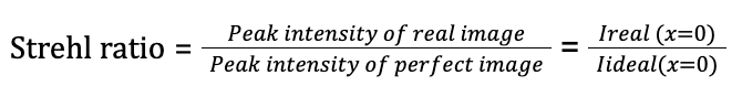
It’s defined using the peak intensity of the image of a point source (the brightness at the very center of the image). This central point corresponds to where the optical axis meets the focal plane for a perfectly aligned (on-axis) punctual light source. As with any measurement performed with our wavefront sensor, the convergent or divergent nature of the analysis beam does not affect the quality of the measurement, provided that it is within the dynamic range of the sensor curvature. If we know the wavefront of the beam at some plane, we can always, with the help of our WaveView software, calculate the PSF by propagating that wavefront to the focal plane. Below is the complex field in an input plane, assume you know the complex field at some plane z=zo.
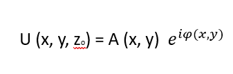
where
- A(x,y) is the amplitude
- ϕ(x,y) is the phase (wavefront)
If the field is known at plane zo, propagation by a distance d is:
Fresnel diffraction (paraxial approximation):

Where k= 2π/λ, ξ and η are coordinates at the plane z=zo, x and y the coordinate at the plane z= zo+d
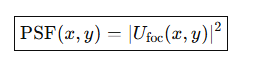
Once you know the complex field at the focal plane, the Point Spread Function or PSF can be derived with the following equation :
This is valid whether the focus is real (converging rays physically meet) or virtual (rays diverge as if from a point). The propagation integral has no distinction, it gives the correct intensity distribution.
The graph below shows how optical aberrations affect image sharpness.
The one curve represents a perfect (non-aberrated) system, with a strong and narrow intensity peak. The other curve shows the aberrated case, where the peak is lower and wider.
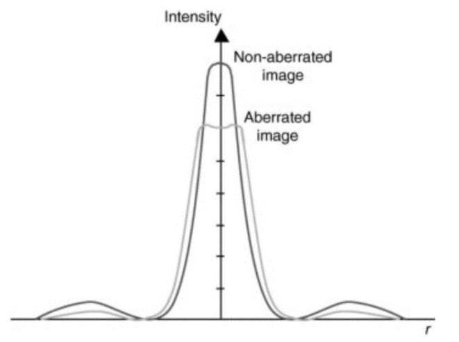
Figure 1: Where x is the position vector, Ireal(x=0) is the maximum of the measured Point Spread Function and Iideal(x=0) is the maximum of the diffracted PSF.
Optimizing Optical Systems: The Power of Strehl and RMS Wavefront Analysis
The Strehl ratio is linked to the wavefront, which ideally should be a perfect sphere or flat. Any small departures from this perfect shape, called aberrations, introduce slight phase errors in the light waves. These errors affect how the waves interfere with each other and change the diffraction pattern that forms the image.
We quantify these imperfections using the RMS (root-mean-square) wavefront error, which shows how much the actual wavefront deviates, on average, from the ideal shape. For small errors (around 0.15 wavelength RMS), the Strehl ratio closely matches how much the optical system’s energy distribution changes. However, this relationship can vary depending on the type and size of the aberrations present.
The Strehl ratio can be approximated by using RMS wavefront values with the expression by Marajal (2)
S ≈ exp[- (2πσω)2≈ 1e2πω2
Where e is the natural logarithm base (2.72) and 𝛚 is the RMS wavefront error in unit of the wavelength.
The graph below presents this approximation of the Strehl ratio as a function of RMS wavefront error. It illustrates how the formula closely follows the exact behavior for small errors.
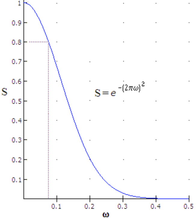
Figure 2: This approximation is accurate to a couple of % for errors of ∽ 1/10 wave. This error increases with the RMS error but even at S~0.3 still doesn’t exceed 10%.
From Lab to Reality: Our AO System predicts Strehl Ratio and PSF Accurately Under Real Conditions
In high-precision optical systems, true performance is measured not only by theoretical calculations but by how closely those calculations match reality. With our Adaptive Optics (AO) platform which combines our HASO-first wavefront sensor with the muDM deformable mirror, we set out to demonstrate exactly that: how accurately our software predicts the Point Spread Function (PSF) and Strehl ratio, and how perfectly the corrected beam aligns with the ideal diffraction-limited spot.
1. Software-Calculated Accuracy: When Theory Meets Reality
One of the core strengths of our system is the precision of our PSF and Strehl ratio calculations. Our WaveTune software reconstructs the expected diffraction-limited PSF based on wavefront measurements and system parameters. But the real validation comes from direct comparison with the far-field camera, which captures the actual intensity distribution of the beam.
What we see is striking:
The calculated PSF profile closely matches the real PSF recorded by the camera, confirming both the reliability of our numerical model and the quality of our wavefront sensing.
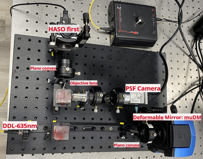
Figure 3: Representation of the adaptive optics (HASO-first, muDM) bench featuring a 10× beam-magnifying objective lens and a high-accuracy HASO-First wavefront sensor
Here are the results from the PSF calculated by our WaveTune software, shown alongside the measured far-field PSF captured by the camera, for an aberrated (uncorrected) wavefront.
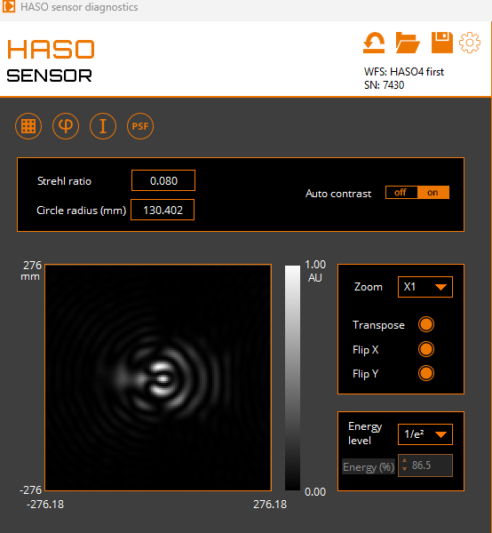
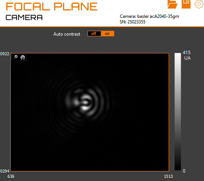
Figure 4: The computed point spread function is shown on the left, while the camera-measured PSF appears on the right. The wavefront is highly aberrated, resulting in a Strehl ratio of less than 0.1
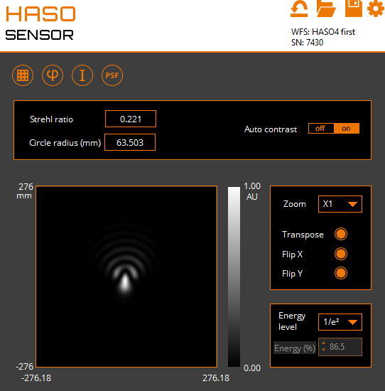
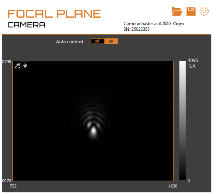
Figure 5: The computed point spread function is shown on the left, while the camera-measured PSF appears on the right. The wavefront is highly aberrated, resulting in a Strehl ratio of 0.221
Here are the results from the PSF calculated by our WaveTune software, shown alongside the measured far-field PSF captured by the camera, for the corrected wavefront.
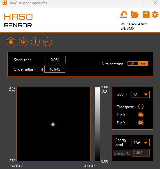
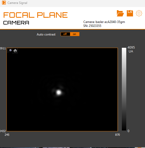
Figure 6:Compares the computed point spread function (left) with the camera-measured PSF (right). The system operates close to diffraction-limited performance, with a Strehl ratio of 0.951.
The measurements clearly demonstrate the precision of our optical system and its ability to correct a strongly aberrated incoming wavefront. Before correction, the system exhibits a significantly degraded PSF with a Strehl ratio of only 0.221 and 0.08, indicating a highly distorted intensity distribution. After applying the correction, the recorded PSF shows a dramatic improvement: the central intensity peak becomes sharp, symmetric, and closely resembles the ideal diffraction-limited profile, yielding a Strehl ratio of approximately 0.951.
The excellent agreement between the Strehl ratio obtained from the PSF camera and the value inferred from the reconstructed wavefront confirms that both diagnostics capture the same physical improvement in image quality. Together, these results verify that our setup not only compensates the initial aberrations effectively, but also restores the system performance to nearly diffraction-limited conditions.
2. After AO Correction: Live Representation of the Nearly Perfect PSF
Once the adaptive correction is applied, the transformation is remarkable.
The PSF evolves from a distorted, broadened distribution into a sharp, symmetric, high-contrast diffraction-limited spot. Both the camera-acquired PSF and the software-calculated PSF converge toward an almost identical, clean Airy pattern.
This not only highlights the strength of the AO correction but also emphasizes the precision with which our software captures and predicts system performance.
Figure 7: Here is a small video showing the aberration correction in real time, with the calculated image on the left and the camera image on the right.
Our Wavefront Metrology software WaveView also reconstructs the corresponding PSF directly from the measured wavefront, allowing us to visualize the beam’s intensity distribution in real time. With WaveView, we can display the x- and y-intensity profiles of the corrected beam live, providing an immediate and intuitive view of how the AO-corrected wavefront translates into the final PSF. This real-time PSF reconstruction offers a clear visual confirmation of the beam quality achieved by the system.
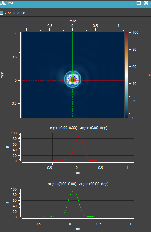
Figure 8: PSF profiles in live
Conclusion:
The comparison between WaveTune-calculated PSFs and the measured far-field camera data demonstrates more than just agreement, it proves the reliability, precision, and real-world readiness of our Adaptive Optics solution. From accurately modeling aberrated wavefronts to delivering a perfectly corrected diffraction-limited spot, the system performs exactly as predicted by our software analytics. The near-perfect overlap between simulated and measured PSFs, both before and after correction, confirms that users can trust every Strehl ratio, every PSF plot, and every performance metric generated by our platform. Whether for demanding research applications or advanced industrial optics, our AO system provides the clarity, accuracy, and confidence needed to reach true peak optical performance.
For more Information on wavefront sensors, click here
For more information on adaptive optics solutions, click here
You can also visit our laser beam diagnostics and Msquared measurements product collections.