
Spatial light modulators (SLMs) give adaptive optics something a fixed optic cannot: programmable, pixel-level control of the phase, amplitude, or polarization of a beam across a two-dimensional plane. Deformable mirrors (DMs) remain the standard for fast, continuous wavefront correction through a physically deformable surface. An SLM is the complementary tool, adding spatial resolution, flexibility, and easy integration, especially for complex wavefront shaping.
In this lab test, we put the Holoeye ERIS-1.1 phase-only LCOS SLM through an aberration-control workout. We wrote known aberrations onto the SLM with Holoeye’s software and measured the resulting wavefronts with a high-resolution LIFT wavefront sensor from Imagine Optic. The result is a quantitative picture of how well an SLM compensates optical aberrations, which matters in applications from high-resolution microscopy and laser material processing to astronomical imaging.
Key results
What a Spatial Light Modulator Does in Adaptive Optics
An adaptive optics system has three jobs: measure the wavefront, compute a correction, and apply it. The corrector is often a deformable mirror, whose continuous reflective surface is pushed and pulled by tens of actuators. A liquid crystal on silicon (LCOS) SLM takes a different route. Each of its pixels holds a liquid crystal layer whose effective refractive index follows the applied voltage, so every pixel adds its own programmable phase delay to the light it reflects.
That pixel-level control is why SLMs excel at complex wavefront shaping. It does not, on its own, guarantee accuracy. Before an SLM can be trusted as a corrector, three questions need answers: how flat is it when nothing is written, does it produce the aberration it is asked for and nothing else, and does its response scale linearly? This test answers all three, then pushes into vortex beams to probe fine phase control.
- Resolution
- 1920 × 1200
- Pixel pitch
- 8.0 µm
- Fill factor
- >95%
- Active area
- 15.42 × 9.66 mm
- Addressing
- 8-bit or 10-bit
- Input frame rate
- 60 / 120 Hz
- Interface
- HDMI + USB
- Display type
- Analog
The 4f Test Bench: How We Measured SLM Aberration Control
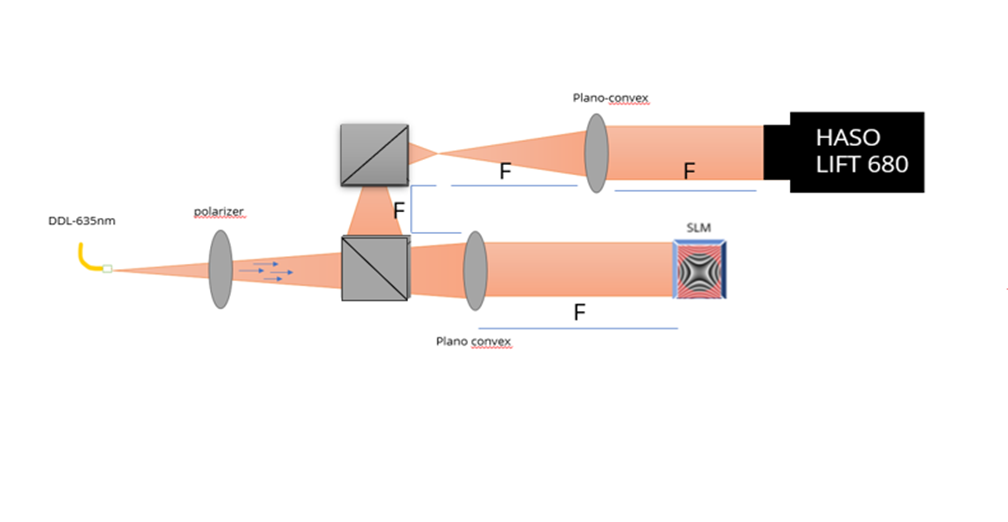
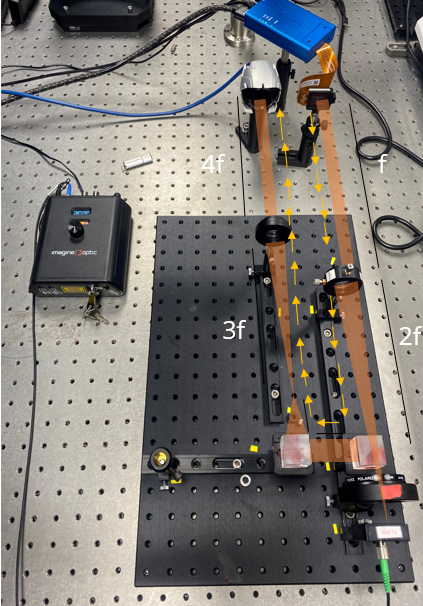
We built a high-precision bench around a 4f imaging relay so wavefront aberrations could be imaged and analyzed accurately. The relay conjugates the SLM plane onto the pupil of a high-accuracy Imagine Optic wavefront sensor, which captures fine phase distortions across the optical field. The same platform supports aberration correction, beam shaping, and adaptive optics work.
Inside the 4f test bench
Select a component to see the role it plays in the measurement.
Collimated laser source. A collimated, linearly polarized beam at 675 nm enters the bench. Starting collimated means any curvature the sensor reports comes from the SLM, not from the source.
Linear polarizer. Liquid crystal SLMs modulate only linearly polarized light aligned with the panel’s specified axis. The polarizer sets that axis so the SLM behaves as a pure phase modulator.
Holoeye ERIS-1.1 phase-only LCOS SLM. 1920 × 1200 pixels at 8.0 µm pitch, driven as a second display over HDMI with calibration over USB. We loaded the Holoeye-supplied calibration file before every measurement. The SLM is reflective; the diagram unfolds it for clarity.
Lens pair forming the 4f relay. Two lenses separated by the sum of their focal lengths image the SLM plane onto the sensor pupil. Because the two planes are conjugate, the sensor reads the phase written on the SLM directly, without the propagation that would blur fine structure such as a vortex core.
Imagine Optic LIFT wavefront sensor. The high-resolution LIFT wavefront sensor measures the phase across the relayed pupil. WaveView software decomposes each map into Zernike coefficients with RMS normalization, and its double-pass tool handles the reflective SLM geometry.
Simplified, unfolded schematic. Figures 1a and 1b show the actual setup.
Test protocol, step by step
1Build the 4f relay
Conjugate the SLM plane to the wavefront sensor pupil with a two-lens 4f relay, and set linear polarization along the SLM’s specified axis.
2Load the calibration
Load the Holoeye-supplied calibration file so the gray-level-to-phase response is linear at the working wavelength.
3Measure the best flat
Command a uniform phase and record the residual wavefront with the WaveView double-pass tool. This is the reference for every later measurement.
4Write single Zernike modes
Write astigmatism, coma, and trefoil one at a time with Holoeye’s software and check the WaveView modal list for one dominant coefficient.
5Double the amplitude
Repeat each mode at twice the commanded amplitude and confirm the measured coefficient doubles while the other modes stay put.
6Write vortex phases
Write helical phase ramps of increasing topological charge and compare the measured peak-to-valley with m waves.
SLM Best Flat: 19 nm RMS Residual Wavefront Error
Spatial light modulators control the phase or amplitude of light pixel by pixel, which makes them highly versatile in advanced optical systems. For many high-precision applications, though, modulation range matters less than intrinsic flatness. The key figure of merit for any wavefront modulator is its best flat: the residual wavefront error left when the device is commanded to a uniform phase. As a rule of thumb, a component whose best flat stays below λ/20 RMS will not degrade the performance of the optical system it sits in.
Holoeye calibrates its SLMs in-house and supplies a calibration file with each device, which we used in this test. An SLM that produces a uniformly flat wavefront, through its physical surface quality or through digital compensation, enables the accurate and repeatable phase modulation that high-fidelity optical control depends on.
We measured with the double-pass tool in WaveView software, treating the SLM as a reflective element. In this configuration, the wavefront generated by the SLM always shows a phase shift or amplitude change that is half of the applied shape.
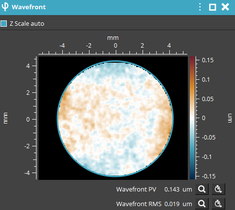
The residual came in at just 19 nm RMS across an 8.5 mm aperture. At the 675 nm wavelength used on this bench, that is roughly λ/35, comfortably inside the λ/20 criterion. Near-flat performance like this supports high-resolution microscopy, optical trapping, adaptive optics in astronomy, wavefront correction in retinal imaging, and laser beam shaping. For comparison, a membrane-based deformable mirror such as the µDM typically achieves a best flat better than 10 nm RMS.
Residual budget calculator
See what a best-flat residual means at your wavelength: the fraction of a wave, the margin against λ/20, and the Strehl ratio the residual implies on its own.
ERIS-1.1 SLM, measured best flat. At 450 nm, 19 nm RMS is 0.042 waves, inside the λ/20 criterion with 3.5 nm to spare.
ERIS-1.1 SLM, measured best flat. At 488 nm, 19 nm RMS is 0.039 waves, inside the λ/20 criterion with 5.4 nm to spare.
ERIS-1.1 SLM, measured best flat. At 532 nm, 19 nm RMS is 0.036 waves, inside the λ/20 criterion with 7.6 nm to spare.
ERIS-1.1 SLM, measured best flat. At 633 nm, 19 nm RMS is 0.030 waves, inside the λ/20 criterion with 12.6 nm to spare.
ERIS-1.1 SLM, measured best flat. At 675 nm, 19 nm RMS is 0.028 waves, inside the λ/20 criterion with 14.8 nm to spare.
ERIS-1.1 SLM, measured best flat. At 780 nm, 19 nm RMS is 0.024 waves, inside the λ/20 criterion with 20.0 nm to spare.
ERIS-1.1 SLM, measured best flat. At 850 nm, 19 nm RMS is 0.022 waves, inside the λ/20 criterion with 23.5 nm to spare.
ERIS-1.1 SLM, measured best flat. At 1064 nm, 19 nm RMS is 0.018 waves, inside the λ/20 criterion with 34.2 nm to spare.
µDM deformable mirror, typical best flat. At 450 nm, 10 nm RMS is 0.022 waves, inside the λ/20 criterion with 12.5 nm to spare.
µDM deformable mirror, typical best flat. At 488 nm, 10 nm RMS is 0.020 waves, inside the λ/20 criterion with 14.4 nm to spare.
µDM deformable mirror, typical best flat. At 532 nm, 10 nm RMS is 0.019 waves, inside the λ/20 criterion with 16.6 nm to spare.
µDM deformable mirror, typical best flat. At 633 nm, 10 nm RMS is 0.016 waves, inside the λ/20 criterion with 21.6 nm to spare.
µDM deformable mirror, typical best flat. At 675 nm, 10 nm RMS is 0.015 waves, inside the λ/20 criterion with 23.8 nm to spare.
µDM deformable mirror, typical best flat. At 780 nm, 10 nm RMS is 0.013 waves, inside the λ/20 criterion with 29.0 nm to spare.
µDM deformable mirror, typical best flat. At 850 nm, 10 nm RMS is 0.012 waves, inside the λ/20 criterion with 32.5 nm to spare.
µDM deformable mirror, typical best flat. At 1064 nm, 10 nm RMS is 0.009 waves, inside the λ/20 criterion with 43.2 nm to spare.
Strehl uses the Maréchal approximation, S ≈ exp[−(2πσ/λ)²]. The calculator holds the residual fixed in nanometers. LCOS SLMs are calibrated per wavelength, and the broadband ERIS-1.1 version covers 420 to 1100 nm, so confirm the best flat at your operating wavelength. The µDM value is the typical best flat quoted for that mirror, not a measurement from this bench.
Generating Zernike Aberrations on Demand: Selectivity and Linearity
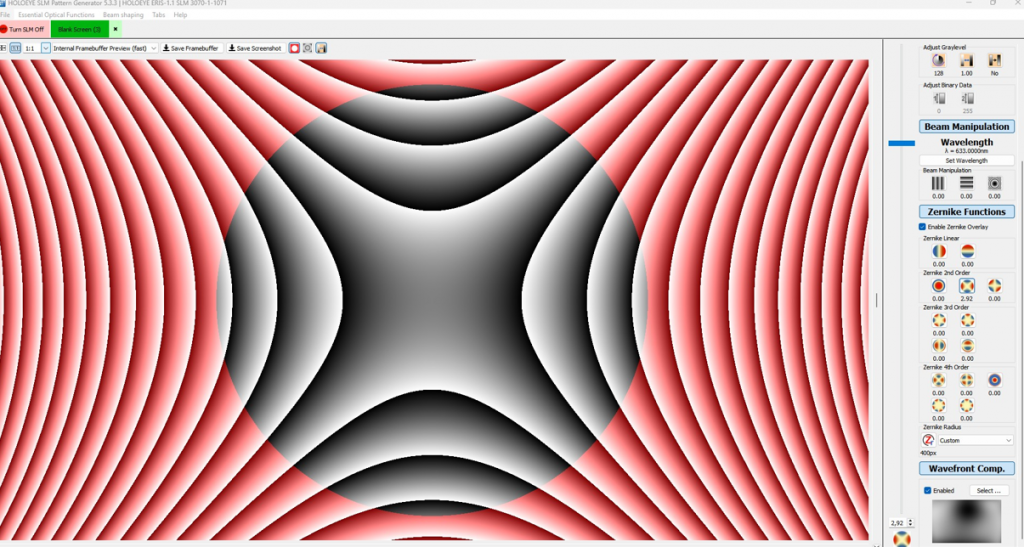
Starting from a flat wavefront, we introduced individual optical aberrations with the SLM, one at a time. WaveView decomposes each measured wavefront into Zernike polynomials with RMS normalization and lists the coefficients in a modal list beside the wavefront map. That list makes cross-talk easy to spot: a clean modulator shows one dominant coefficient for the introduced mode and minimal values for the rest.
Aberration explorer
Write a mode to the SLM, then double it. The map and modal list update the way they did in WaveView.
Maps and bars are schematic, drawn on a fixed color scale so the 2× state reads twice as strong. The measured WaveView result for the selected mode is shown below.
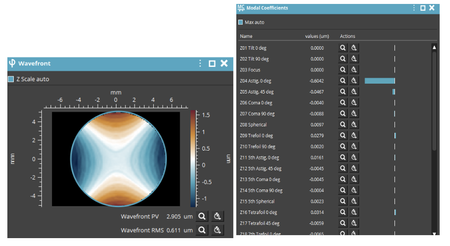
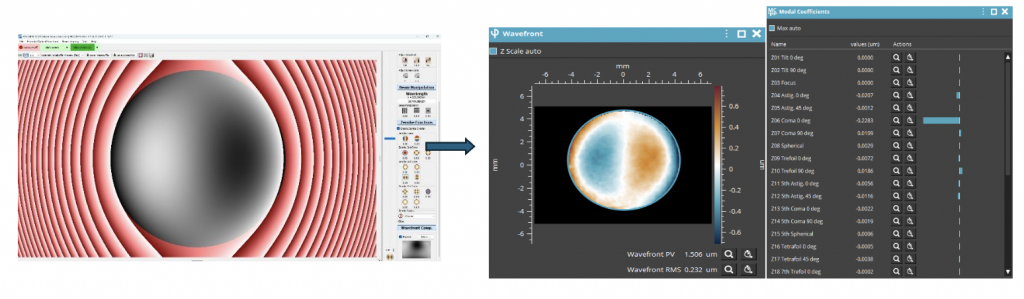
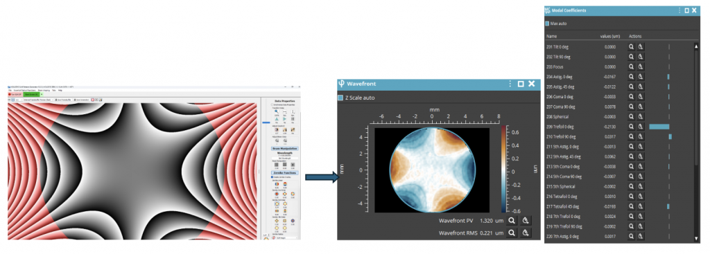
Every aberration we introduced appeared distinct and well isolated, with a dominant coefficient for the requested mode while the others remained minimal. The SLM also proved linear: when the amplitude of a given aberration was doubled on the SLM, the response measured on the sensor was twice the initial value. Selectivity and linearity together are what make an SLM usable as a corrector, because a control loop assumes each command produces a predictable, proportional change in one mode only.
Vortex Beam Generation with an LCOS SLM
Here the difference between an SLM and a deformable mirror becomes concrete. A deformable mirror shapes light through continuous surface deformation, while an SLM sets the phase in discrete, pixel-level steps. That discrete control lets an SLM write complex phase patterns such as optical vortex beams, which carry orbital angular momentum (OAM).
A vortex beam needs precise azimuthal phase modulation: a helical phase ramp that winds through m full cycles of 2π around a central singularity, where m is the topological charge. Measured with a wavefront sensor, an ideal helix shows a peak-to-valley of m·λ around the vortex, so the measurement doubles as a check on how continuous and uniform the phase variation is across the full angular span. We introduced a range of topological charges and measured the resulting phase profiles with the wavefront sensor.
Vortex beam explorer
Pick a topological charge. The phase wraps m times around the core, the ring widens, and the expected wavefront peak-to-valley grows by one wave per unit of charge.
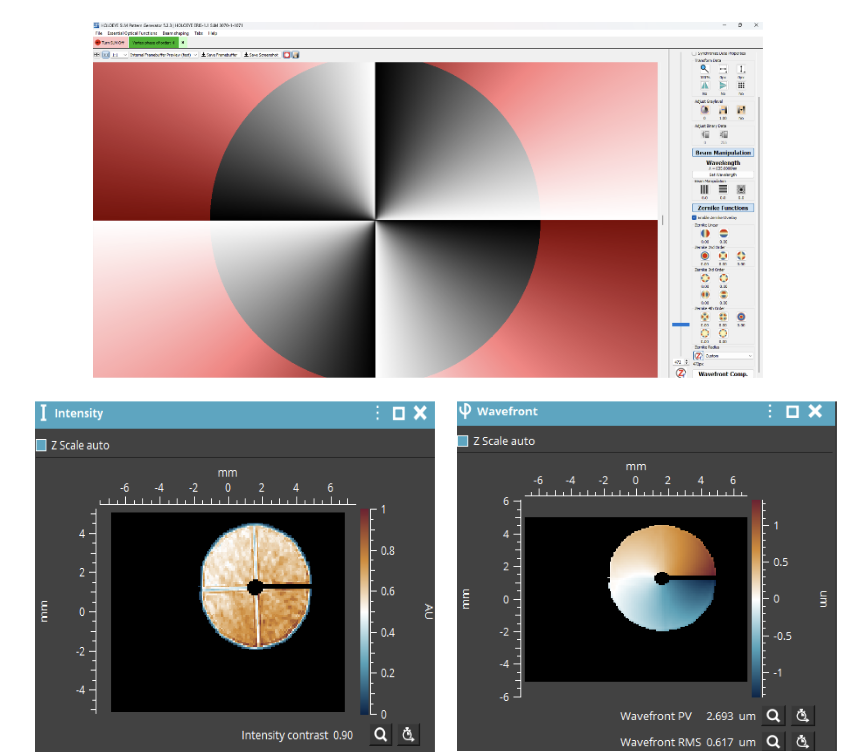
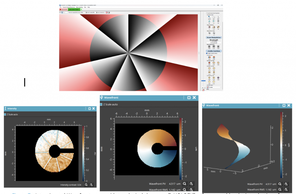
Phase and intensity tiles are ideal Laguerre-Gaussian (p = 0) profiles at a fixed waist w, for illustration. Measured values come from the LIFT sensor at 675 nm.
Both measured charges land close to their integer targets: 2.693 µm of peak-to-valley for m = 4 is 3.99 waves at 675 nm, and 4.517 µm for m = 7 is 6.69 waves. Holding a clean helical ramp at m = 7, where the phase cycles seven times around the core, demonstrates the fine phase control and beam-shaping capability that set an SLM apart. Holoeye software makes high topological charges easy to introduce, and a high-accuracy wavefront sensor makes them precise to verify.
SLM or Deformable Mirror for Aberration Correction?
The two correctors are complementary rather than competing. The short version:
| Factor | LCOS spatial light modulator | Deformable mirror |
|---|---|---|
| Control elements | Millions of pixels, discrete phase steps | Tens of actuators, continuous surface |
| Best at | High spatial resolution, holograms, multi-spot patterns, vortex beams | Large stroke, speed, high laser power |
| Wavelength | Calibrated per wavelength band | Achromatic |
| Polarization | Linear, aligned to the panel axis | Polarization independent |
| Best flat in this test | 19 nm RMS (ERIS-1.1, measured) | <10 nm RMS typical (µDM) |
For a full comparison with an interactive selector, read our deformable mirror vs. spatial light modulator guide, or browse the deformable mirror and spatial light modulator lineups.
Where SLM-Based Aberration Control Is Used
Microscopy
Correct sample-induced aberrations to restore resolution and signal in advanced light microscopy.
Optical trapping
Shape and steer multiple traps from one beam for optical tweezers.
Astronomy and FSO
Compensate atmospheric turbulence for telescopes and free-space links, as with CIAO.
Retinal imaging
Correct the eye’s aberrations to resolve fine structures in the retina.
Laser beam shaping
Form top-hat, Bessel, Airy, and custom profiles for laser beam shaping.
Holography and OAM
Generate computer-generated holograms, higher-order modes, and OAM beams.
From Validation to Closed-Loop Adaptive Optics
The results confirm the high precision and reliability of the SLM for accurate, selective wavefront control. It delivered excellent linearity, stability, and very low cross-talk across every aberration and beam shape we introduced, including vortex beams. Those capabilities validate it for high-performance optical applications that need dynamic phase modulation.
Our next step, in a future post, is to integrate the SLM as the corrective element in a closed-loop adaptive optics system. If you are building that loop now, the AO Kit SLM packages SLM-based adaptive optics as a kit, WaveTune adaptive optics software drives deformable mirrors and spatial light modulators alike, and the WaveKit SDK exposes Python, C++, and LabVIEW interfaces for custom control.
Planning an SLM or adaptive optics setup?Our applications team can help you match the modulator, wavefront sensor, and software to your wavelength, aperture, and correction speed.
Spatial Light Modulator FAQs
What does a spatial light modulator do in adaptive optics?
A spatial light modulator (SLM) applies a programmable phase delay pixel by pixel across a beam. In adaptive optics it acts as the wavefront corrector, writing the inverse of a measured aberration so the outgoing wavefront is flat. Phase-only LCOS SLMs such as the Holoeye ERIS-1.1 offer millions of independently addressable pixels, which suits complex, high-resolution wavefront shaping.
How flat is an LCOS spatial light modulator?
With the manufacturer calibration file loaded, the ERIS-1.1 we tested reached a best flat of 19 nm RMS residual wavefront error across an 8.5 mm aperture. At the 675 nm test wavelength that is about λ/35, well inside the common λ/20 RMS criterion for a component that will not degrade system performance.
Does an SLM respond linearly to commanded aberrations?
Yes, in our test. Each Zernike aberration written to the SLM appeared as a dominant coefficient for that mode with minimal cross-talk into others, and doubling the commanded amplitude doubled the coefficient measured on the wavefront sensor. Linear, selective response is what a closed-loop adaptive optics controller relies on.
Can a spatial light modulator generate vortex beams?
Yes. Because an SLM controls phase pixel by pixel, it can write the helical phase ramp of an optical vortex, which carries orbital angular momentum. We generated vortex beams with topological charges m = 4 and m = 7 and measured wavefront peak-to-valley values of 3.99 and 6.69 waves at 675 nm, close to the ideal m waves.
Why use a 4f imaging relay to test an SLM?
A 4f relay makes the SLM plane and the wavefront sensor pupil optically conjugate, so the sensor measures the phase written on the SLM directly rather than a version altered by free-space propagation. That keeps fine structure, such as the core of a vortex beam, intact for measurement.
Do spatial light modulators require polarized light?
Liquid crystal SLMs modulate only linearly polarized light aligned with the panel’s specified axis, which is why the test bench places a linear polarizer ahead of the SLM. Deformable mirrors, by contrast, are polarization independent.
Should I use an SLM or a deformable mirror for aberration correction?
Choose a deformable mirror when the priority is large stroke, speed, broadband or multi-wavelength operation, polarization independence, or high laser power. Choose an SLM when you need high spatial resolution or complex light fields such as holograms, multi-spot patterns, and vortex beams. Our deformable mirror vs. spatial light modulator guide compares the two in detail.
What software drives the Holoeye ERIS-1.1 SLM?
The ERIS-1.1 connects over HDMI and runs as a secondary display, with a USB link for calibration. Holoeye supplies a Pattern Generator for lenses, gratings, axicons, vortex functions, and computer-generated holograms, plus an SLM Display SDK with APIs for LabVIEW, MATLAB, Octave, Python, and C or C++.