


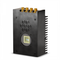

pSPAD | Photon-Counting & Time-Stamping SPAD Arrays
Sensor Technology
SPAD
Quantum Efficiency
50% - 62%
Readout Noise
0 e- rms
Sensor Resolution
23 / 25 / 93
Readout Rate
180 MHz / 310 MHz / 3,560 MHz
Time-Tagging Resolution
20 ps
 Description
 Specifications
 QE Curve
 Applications
 Pictures
 Videos
 Downloads
 Publications
SPAD23 photon-counting SPAD array, in a nutshell
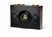
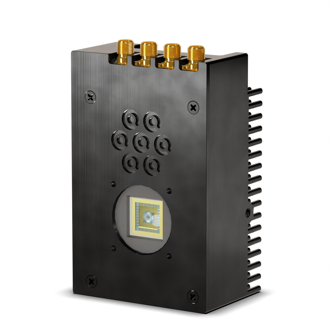
SPAD23 is a photon-counting array with 23 hexagonally packed single-photon avalanche diodes (SPADs) with best-in-class performance. SPAD23 is based on proprietary SPAD chips with optimized pixels for high sensitivity and low noise. It enables a peak photon detection probability of more than 50%, a typical dark count rate of less than 100 counts per second and literally zero readout noise.
SPAD23 enables photon counting at a maximum rate of 7.8 M counts per second, and time tagging with a resolution down to 20 ps and software control can be accessed through TCP/IP for easy integration into LabVIEW, Matlab, or Python.
What is a SPAD or single-photon avalanche diode ?
A single-photon avalanche diode or SPAD is a solid-state photodetector based on a reverse biased semi-conductor p-n junction like photodiodes and avalanche photodiodes (APDs), but unlike regular photodiodes, a SPAD operates in a mode called “Geiger mode” where a single incoming photon will create an electron-hole pair which will be amplified enough to create a measurable current. Therefore SPADs are intrinsically able to detect single-photons, with a very high temporal resolution.
The key component of a SPAD is a region within the diode called the depletion region. This region is designed to have a high electric field, which allows it to function as a high-gain avalanche photodiode. When a single photon interacts with the depletion region, it generates an electron-hole pair. The high electric field across the depletion region causes the electron and hole to accelerate, leading to a process known as impact ionization in which each electron or hole can gain enough energy to generate another electron-hole pair, resulting in an avalanche effect. This avalanche process rapidly amplifies the initial signal, converting the weak optical signal from the single photon into a detectable electrical pulse.
SPADs can be compared to other single-photon detection technologies such as PMTs and APDs, but SPADs have several advantages over those two type of detectors.
Compared to photomultiplier tubes (PMTs), SPADs have:
- higher sensitivity over wider spectral range ;
- better time resolution ;
- less bulky so more suitable for assembling into large arrays ;
- less sensitive to electromagnetic or mechanical perturbations.
Compared to avalanche photodiodes (APDs), SPADs have:
- higher detection efficiency
- smaller active areas
- generate less dark counts.
What is a SPAD array ?
A SPAD array refers to an arrangement of multiple single-photon avalanche diodes (SPADs) that are integrated into a two-dimensional array format. Each SPAD within the array operates independently and is capable of detecting individual photons. The SPAD array combines the sensitivity and photon-counting capabilities of SPADs with the ability to detect photons across a larger spatial area.
Each SPAD in the array is assigned a unique address, allowing individual SPADs to be accessed and controlled independently. This addressing scheme enables selective readout of specific SPADs or groups of SPADs within the array, providing flexibility in data acquisition and analysis.
The main advantage of using a SPAD array is the ability to perform spatially resolved photon detection. By detecting photons across multiple locations simultaneously, it allows for the capture of detailed spatial information about the incoming light. This is particularly useful in applications such as imaging, where the spatial distribution of photons can be used to construct images or maps.
To view more photon counting cameras, click HERE.

Confocal Microscopy: ISM, FLIM & STED


SPAD 23 Software
Downloads
Go to https://www.piimaging.com/docs/ to download the latest software versions for both Windows and Linux. Both software versions should run standalone and feature the same functionalities. The Windows version has been tested on Windows 10 and 11. The Linux version is tested on Ubuntu 20.04 and 22.04.
Installation
Windows:
- Unzip the downloaded package. It contains the following folders:
- Drivers
- SPAD23_standalone_win64
- Install the drivers and the Visual C++ Redistributables from the Drivers folder.
- Connect the two USB-C cable to the camera.
- Connect the 5V power plug to the camera.
- Run the software by double clicking the SPAD23.exe in the SPAD23_standalone_win64 folder.
- You should now be able to see the live view with the photon counts in each detector.
Linux:
- Unzip the downloaded package. It contains the following folders:
- Install
- SPAD23_standalone_linux64
- Open a terminal in the Install folder and execute the following command: sudo ./install.sh . You might be prompted for your administrator password to proceed with the installation. The installation file might require execution permissions, set this with sudo chmod +x install.sh .
- Connect the two USB-c cable to the camera.
- Connect the 5V power plug to the camera.
- Run the software by double clicking the SPAD23 executable in the SPAD23_standalone_linux64 folder. Alternatively, open a terminal in the SPAD23_standalone_linux64 folder and execute: ./SPAD23 . The application might require execution permissions, set this with sudo chmod +x SPAD23 .
- You should now be able to see the live view with the photon counts in each detector.
Setting up
Graphical User Interface (GUI)
Menu
The options menu is available in the top left corner of the user interface. There are the following options:
- Toggle live view to linear/log > Switch between the display of the count rate in the live views in a linear or logarithmic fashion.
- Toggle histogram to linear/log [TDC version] > Switch the histogram displayed on the timestamping tab to have either a linear or logarithmic y-axis.
- Change clock SMA mapping > Opens a secondary window in which the user can reassign the SMA ports to a different frame/line/dwell clock.
- Disable/enable VOP > Turn on and off the detectors high-voltage supply.
- Disable/enable dummy clock markers > By default the firmware will not generate dummy clock markers for frame/line/dwell clocks. However, for debugging purposes, the internal generation of dummy markers can be activated with this toggle.
- Check for updates > Forces an online check for a new software version.
- Help > Opens this online documentation portal.
- Quit > Closes the software and reduces the SPAD operating voltage to a save condition.
Live view
The live view tab shows a graphical representation of the current photon counts on the 23 SPAD pixels. The view is adjusted proportionally to the brightest pixel, which is completely white. A black—red—yellow—white colour scale shows the intensity variation over the array. Clicking on one of the pixels in the live view will disable the pixel’s visual output. Hovering over any of the pixels will reveal its current count rate in counts per second (cps) in the bottom status bar. Otherwise the integrated photon count rate over the whole array will be displayed.

A small version of the live view is also available on the photoncounting and timestamping tabs in the bottom left corners.
Photoncounting
The second tab provides the photon-counting capabilities of the system. On the left is a control panel to setup the parameters for the measurements that are printed in the window on the right. The measurement progression is indicated in the bottom status bar. The following options are available:
- Classical button > Set the measurement window for classical single-shot intensity measurements.
- Scanning button > Set to scanning mode, this mode allows to continuously measure with the help of the provided line / dwell clocks on the systems SMA connectors. This mode does not function without a line clock!
- Integration time > Set the measurement integration time either in milliseconds for classical operation mode, or microseconds for scanning operation mode.
- The following options are only available in scanning operation mode:
- Frames > Set the number of frames.
- X > Set the number of pixels or dwells in a single line.
- Y > Set the number of lines.
- Ext. dwell clk checkbox > Enable the use of the external dwell clock provided through the SMA connector and override the internal integration time.
- Ext. frame clk checkbox > Enable the use of the external frame clock provided through the SMA connector. The scan will wait at the beginning of each frame for the rising edge of the frame clock.
- Live view checkbox > Enables the live view. In this mode, the system will continuously take a new scan and display the image, until the stop button is pressed.
- Image checkbox > Enable the conversion of the raw data to a set of images.
- Non-scaled checkbox > By default the images will be scaled with respect to the brightest pixel. This box disables scaling. The non-scaled value represents the photon counts with 8-bit counter depth.
- Raw data checkbox > Process and print/save the raw data in text format.
- Save checkbox > Saves the measurements to a file or an image. A folder data/counters is created in the run directory and files are saved with the name Run_classicalXXX.txt, Run_scanningXXX.txt or IMGXXX-YY.png. XXX denotes the run iteration, YY is the pixel number 0—22 and 23 for the combined result.
- Start button > Launches the chosen measurement.

The standard measurement data is formatted with the first column being the pixel number and the second being the measured counts in the given measurement time. The scanning measurement principle is shown below. If the external frame clock is used, the scan will halt at the beginning of each frame, until the rising edge of the frame clock. The rising edge of the next line clock starts the integration of the first dwell of that line, each consecutive rising edge of the dwell clock increments the dwell counter by one. The final dwell in the line is finished at the rising edge of the dwell clock. At the end of the line, the dwell counter is reset to zero and the system waits until the next rising edge of the line clock. Once the system has integrated the requested number of lines, the frame counter is incremented and the system will wait for the next rising edge of the frame clock (if external frame clock is used) or proceed directly to wait for the next rising edge of the line clock.
(0,0,1),6,1,1,1,3,3,7,1,1,0,1,1,3,2,2,2,2,3,4,1,3,1,5
(0,0,2),2,2,2,2,3,0,3,5,4,0,1,3,1,2,2,0,2,3,0,0,6,1,4(1,63,126),0,2,0,4,2,3,2,4,2,0,2,0,2,0,2,1,1,2,1,4,0,2,1
(1,63,127),0,2,1,2,1,3,1,1,1,0,1,3,2,0,1,5,2,1,1,3,6,1,1
The generated image with a size of X* × Y* is displayed on the right hand side of the screen. One can scroll through the frames with the slider on top of the image or play the sequence with the play button. By default, a scaled image with the summation of the pixel counts from all 23 detectors is shown. The generated image for each individual SPAD detector can be displayed by clicking on the pixel in the mini-live view in the left side of the window. When saving, all 23+1 images will be generated in the data/counters folder for each frame.
Timestamping
The third tab gives access to the time-stamping capabilities. This interface is adapted according to the detected firmware version. The first system version features coarse (10 ns) time-stamping. The second has time-to-digital converters (TDCs) with a fine resolution (~10 ps).
Coarse time-stamping:

The control panel on the left has the following options:
- Integration time
Set the measurement integration time in milliseconds. Setting a time equal to zero will start an unlimited time measurement. The measurement can be stopped with a click on the stop button. - Pixels to mask
Set the pixels that are not required, separated with a comma or semicolon:0,1,2,...,22. - Image checkbox
Generate an image for each of the 23 pixels + the combined results (currently the images contain just the intensity information). The 24 images for each frame are written into a new folderdata/tdc/RunXXX. Note that this mode requires a dwell, line and frame trigger to operate successfully. - Raw data checkbox
Save the raw data directly in a new folderdata/timers/RunXXX. - Start button
Launches the chosen measurement.
The progress of the measurement and the processing of the data is shown in the bottom status bar. The measurements are saved to separate files per pixel. A folder data/timers/RunXXX is created in the run directory and files are saved with the name pixXX.txt. Special markers and additional information is saved in pix23.txt, this information is also printed in the right side of the window.
The pixel data is formatted as a single column with the value of the coarse clock counter at the photon arrival time. The real-time streaming data is formatted slightly different, see the Command guide.
The marker data is formatted with the first column being the marker or special event number, which has to be read as follows:
-59— File header-56— Reset of the coarse clock counter, only the wraparound data is printed (when the clock starts at zero again)-17— USB FIFO almost full, send only markers-16— USB FIFO reasonably empty, resume normal operation-12— Frame marker-10— Line marker-9— Dwell marker-0— End of measurement
The second column is the value of the coarse clock counter running at 100.8MHz, i.e. this allows to determine the arrival time down to 10ns.
Fine time-stamping:

Additional options in the control panel:
- TDC setting dropdown box
The operation of the TDC can be selected here, there are three modes.- Calibrate, runs the calibration of the TDCs. Measures the length of the TDC channels and stores them for further measurements.
- SPAD input, normal operation.
- Align pixels, requires a synchronous light source, measures the histograms of all pixels and calculates the rising edge offsets in each TDC channel for alignment of further measurements. The table is stored and loaded on startup.
- Histogram checkbox
Generate and save a histogram from the measurement data for each pixel (the histogram will update at real-time). The data is saved directly in a new folderdata/tdc_hist/RunXXXand the histogram is plotted in the right window. Other pixels can be selected by clicking in the mini-live view on the left. The data is formatted with the first row being the time in picoseconds, all further rows contain the number of counts in that time window and per dwell (if enabled). The first row is saved separately indata/tdc_hist/RunXXX/pixtimeaxis.txtto save space. - Split dwells checkbox
Split the histograms for each new dwell. A slider will be shown to cycle through the dwells. In the output file, the histogram for each dwell will be printed on a new line. Note that this might cause some lag for a dwell amount >2000. - Image checkbox
Generate an image for each of the 23 pixels + the combined results (currently the images contain just the intensity information). The 24 images for each frame are written into a new folderdata/tdc/RunXXX. Note that this mode requires a dwell, line and frame trigger to operate successfully. - Raw data checkbox
Save the raw data directly in a new folderdata/tdc/RunXXX.
Before the first measurement, the TDC needs to be calibrated. The software is already setup in calibration mode, which can be run by simply clicking the play button.
The pixel data is formatted in 2 columns. From left to right they represent:
- The converted TDC result (in picoseconds) with respect to the laser clock.
- The coarse counter value, synchronous with the supplied laser clock.
The format of the marker data is unchanged with respect to the coarse counting system, with the exception of the coarse counter being shorter. Note that the data format for the TCP/IP stream option is slightly different, see the remote command guide section.
Settings
- Top left > Status indication of the USB connection. This is indicated green when the system is connected by USB3. The system can be reinitialized by clicking the reset button. The software gives a warning when the system is not connected with USB3.
- Top middle > Speed test for the USB connection. The transfer speed is calculated by transferring the set number of bytes and dividing by the required time.
- Top right > Pulse width (i.e. the SPAD dead-time) and pulse distance measurements. On the FPGA, a histogram is generated during the set integration time for the selected SPAD pixel. The data is formatted with the first column being the time in nanoseconds, the second being the number of counts in that time window. The data can be saved with the save button into a file
RunXXX.txtin a newdata/debugfolder. With the default operating voltages, the average pulse width should be in the order of 50ns. - Bottom left > Current operating voltages. The operating voltages can be changed on the fly. Vq will automatically be calculated upon changes in VOP to tune the pixel dead-time to a value in the order of 50ns.
- Bottom middle (I) > Current operating temperatures of the FPGA and the PCB on which the sensor is located. Therefore, the PCB temperature should be a good indication of the sensors current operating temperature. Ideally, the sensor temperature should be kept as low as possible. Without air flow, the PCB temperature should be below 40°C.
- Bottom middle (II) > Current SMA input frequencies. Shows the current running frequency for the SMA inputs: laser, frame, line, dwell clock.
- Bottom right > Status of the remote communication server. The software can be programmed from any capable TCP/IP software package, see the command guide for instructions. The listening port on the localhost can be changed through the dropdown menu.